Bounding boxes and hierarchies
This is an online bonus chapter for The Ray Tracer Challenge, by Jamis Buck. To be successful, you:
should have an account at the Ray Tracer Challenge forum. Ask all your questions there, and see how others have managed!
must have a copy of The Ray Tracer Challenge.
must have implemented your ray tracer through chapter 14 (Groups).
If you don't have a copy of the book, grab one today and start writing a 3D renderer of your own!
Your ray tracer probably performs great with the simpler of your test scenes. A plane or two, a handful of spheres, perhaps even a cube or cylinder thrown in for variety—these aren't going to tax your computer terribly. But as soon as your scene grows much bigger than that—and especially if it gets into the hundreds or thousands of elements—you'll find that your renderer begins to bog down, and render times start to drag on into the realm of hours, or even days.
Why? It's because your renderer has to iterate over every object in your scene for each ray it casts, and you'll probably have at least two such rays for each pixel in your image—one for the initial ray, and one for the shadow ray at the point of intersection. Thus, the more objects you have in your scene, the more objects have to be tested for every pixel you render.
Well, then. If you want your renderer to go faster, it becomes a matter of reducing the number of objects that have to be examined at each pixel. Right? The question now is: just how are you supposed to do that?
In this bonus chapter, you'll learn how to optimize large scenes by using bounding boxes and bounding volume hierarchies. By the end, you should see significant improvements when rendering scenes with large numbers of objects, like triangle meshes.
Here we go!
Bounding boxes
Imagine a scene containing a 3D grid of spheres, with 10 spheres on a side.
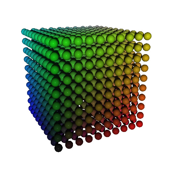
That's, like, a thousand spheres, right? And the way your ray tracer is currently implemented, every ray you cast is going to have to be tested against every single one of those spheres, which means you can expect your render to take roughly...let's see...multiply...carry the one... Um. Let's just call it an eternity.
BUT.
What if you were to put all of those spheres inside a big, invisible box? And then, what if you reworked your ray tracer so that it only tried to intersect the shapes if a ray happened to intersect the box that contained them?

This is what is called a bounding box. Technically, you could use a sphere instead, or a cylinder, or really any other shape, in which case you would talk about bounding volumes instead of bounding boxes. The goal is to pick a relatively simple shape that forms the tightest possible bound on its contents. Boxes (and especially the axis-aligned bounding boxes from chapter 12) work well as a general solution for this, because they are simple to construct and inexpensive to intersect.
So, that's what you're going to build here. The process will look something like this:
- Implement a
BoundingBoxstructure and some associated logic to manipulate it. - Add a function to each primitive shape for querying the shape's bounds (in object space).
- Implement a function for recursively finding the bounds of a
Groupobject. - Implement a function for recursively finding the bounds of a
CSGobject. - Detect if a ray intersects a bounding box.
- Add a guard to the
local_intersect()function of your aggregate shapes (GroupandCSG).
Once you've nailed that down, you'll move on to the second half of this optimization: bounding volume hierarchies, but let's not get ahead of ourselves. First things first: bounding boxes. Onward!
The BoundingBox structure
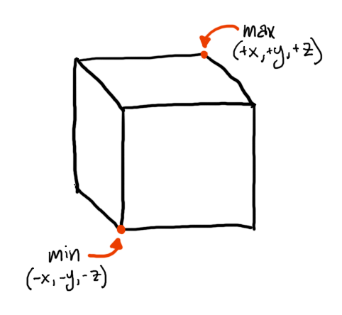
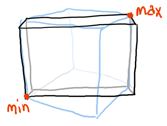
A BoundingBox is a simple structure describing an axis-aligned bounding box, or AABB. It contains just two points, one identifying the minimum point on the box, and the other identifying the maximum point. The minimum point is where the x, y, and z coordinates are all smallest, and the maximum point is where those coordinates are all largest.
Initially, though, the box will be empty, which means its min and max points are a bit wonky by default. The following test demonstrates this:
bounds.featureScenario: Creating an empty bounding box
  Given box ← bounding_box(empty)
  Then box.min = point(infinity, infinity, infinity)
    And box.max = point(-infinity, -infinity, -infinity)
What? Yeah, like I said, wonky. An empty bounding box has it's smallest point at positive infinity, and it's largest point at negative infinity. Basically, what this is saying is that the empty box is invalid. It contains no space whatsoever.
You may be wondering, "why bother with an empty bounding box at all?" It does seem pretty pointless, but hang in there. When you start dealing with adding points to these boxes, or combining multiple boxes together, having your empty boxes start out "wonky" actually makes things easier.
To describe a bounding box that encapsulates some volume, you instantiate the box with explicit minimum and maximum points, like this:
bounds.featureScenario: Creating a bounding box with volume
  Given box ← bounding_box(min=point(-1, -2, -3) max=point(3, 2, 1))
  Then box.min = point(-1, -2, -3)
    And box.max = point(3, 2, 1)
Later in this chapter you'll define several operations on these bounding boxes, but for now, you'll add just one: the ability to resize a bounding box so that it includes a given point. It looks like this:
bounds.featureScenario: Adding points to an empty bounding box
  Given box ← bounding_box(empty)
    And p1 ← point(-5, 2, 0)
    And p2 ← point(7, 0, -3)
  When p1 is added to box
    And p2 is added to box
  Then box.min = point(-5, 0, -3)
    And box.max = point(7, 2, 0)
Every time you add a point to a bounding box, the box adjusts its min and max points, resizing itself so that it can contain the given point. It does this by checking the x, y, and z components against the x, y, and z components of the min and max points. If any component is less than the corresponding component of min, that component of min is replaced with the new value. Similarly, if any component is greater than the corresponding component of max, that component gets replaced. Here's some pseudocode:
# adding "point" to "box"

box.min.x ← point.x if point.x < box.min.x
box.min.y ← point.y if point.y < box.min.y
box.min.z ← point.z if point.z < box.min.z

box.max.x ← point.x if point.x > box.max.x
box.max.y ← point.y if point.y > box.max.y
box.max.z ← point.z if point.z > box.max.z
With that implementation in mind, recall how your empty box was defined: min was positive infinity, and max was negative infinity. This means that any point you try to add to that empty box it will be smaller than min, and larger than max, allowing the pseudocode above to automatically snap your box to the given point. See? Wonky is wonderful!
Once you have that much defined, you can begin describing the bounds for each of the primitive shapes in your ray tracer.
Bounds for primitives
By the time you reach chapter 14, "Groups", of The Ray Tracer Challenge, your ray tracer ought to include the following primitives:
- spheres
- planes
- cubes
- cylinders
- cones
In this section, you'll define bounds for each of those primitive types, as well as triangles. (If you haven't yet reached chapter 15, "Triangles", you can skip that part and come back to it when you're ready.)
For each of these primitive shapes, you'll define a function called bounds_of(shape), which returns a bounding box in object space. This means that, for now, you won't need to worry about any transformations on the objects.
Spheres
The spheres in your ray tracer are always at the origin, and have a radius of 1. This means that the corresponding bounding boxes will also be centered at the origin, and extend from -1 to 1 along each axis.
spheres.featureScenario: A sphere has a bounding box
  Given shape ← sphere()
  When box ← bounds_of(shape)
  Then box.min = point(-1, -1, -1)
    And box.max = point(1, 1, 1)
Planes
Planes are trickier, because they stretch to infinity in x and z, and have zero thickness in y.
planes.featureScenario: A plane has a bounding box
  Given shape ← plane()
  When box ← bounds_of(shape)
  Then box.min = point(-infinity, 0, -infinity)
    And box.max = point(infinity, 0, infinity)
Any bounds you wrap around a plane are effectively useless, because even the tiniest rotation will cause it's bounding box to suddenly stretch to infinity along every axis. Still, having a bounding box defined for it helps avoid special cases, so it's worth doing.
Cubes
Cubes are great, because they can be perfectly bound by their bounding box. There is literally no other shape that bounds a cube more effectively than another cube of the same shape and size.
cubes.featureScenario: A cube has a bounding box
  Given shape ← cube()
  When box ← bounds_of(shape)
  Then box.min = point(-1, -1, -1)
    And box.max = point(1, 1, 1)
Neat, huh?
Cylinders
Like planes, an infinite cylinder (or cone) is kind of worthless when it comes to trying to bound it, because any rotation will cause it to expand to infinity. For completeness, though, it's worth defining anyway.
In object space, the cylinder extends from -1 to 1 in both x and z, and from -infinity to infinity in y:
cylinders.featureScenario: An unbounded cylinder has a bounding box
  Given shape ← cylinder()
  When box ← bounds_of(shape)
  Then box.min = point(-1, -infinity, -1)
    And box.max = point(1, infinity, 1)
Once you limit the cylinder (and especially if you limit it at both ends), it becomes much easier to bound:
cylinders.featureScenario: A bounded cylinder has a bounding box
  Given shape ← cylinder()
    And shape.minimum ← -5
    And shape.maximum ← 3
  When box ← bounds_of(shape)
  Then box.min = point(-1, -5, -1)
    And box.max = point(1, 3, 1)
Cones
Bounding boxes around infinite cones are perhaps the most useless of all, because cones extends to infinity along every axis.
cones.featureScenario: An unbounded cone has a bounding box
  Given shape ← cone()
  When box ← bounds_of(shape)
  Then box.min = point(-infinity, -infinity, -infinity)
    And box.max = point(infinity, infinity, infinity)
Limiting the cones makes them easier to bound, though the logic is more complicated than you might think at first glance.
cones.featureScenario: A bounded cone has a bounding box
  Given shape ← cone()
    And shape.minimum ← -5
    And shape.maximum ← 3
  When box ← bounds_of(shape)
  Then box.min = point(-5, -5, -5)
    And box.max = point(5, 3, 5)
To find the bounds of a limited cone, choose the largest of the absolute values of cone.minimum and cone.maximum. Call it limit. The cone's bounding box then goes from -limit to limit in both x and z, and from cone.minimum to cone.maximum in y.
In pseudocode:
function bounds_of(cone)
  let a ← abs(cone.minimum)
  let b ← abs(cone.maximum)
  let limit ← max(a, b)

  return bounding_box(min=point(-limit, cone.minimum, -limit)
                      max=point(limit, cone.maximum, limit))
end function
Triangles
Finding the bounding box for a triangle is a matter of finding the smallest and largest x, y, and z components from its three points.
triangles.featureScenario: A triangle has a bounding box
  Given p1 ← point(-3, 7, 2)
    And p2 ← point(6, 2, -4)
    And p3 ← point(2, -1, -1)
    And shape ← triangle(p1, p2, p3)
  When box ← bounds_of(shape)
  Then box.min = point(-3, -1, -4)
    And box.max = point(6, 7, 2)
The (conceptually) simplest way to implement this is to just declare an empty bounding box, and then add each of the triangle's points to it:
function bounds_of(triangle)
  let box ← bounding_box(empty)

  add triangle.p1 to box
  add triangle.p2 to box
  add triangle.p3 to box

  return box
end function
And there you have it!
The Test Shape
Lastly, it may seem odd to put bounds on an abstract shape that you only use in tests, but it'll be useful for some of the tests later in this chapter. For the sake of test_shape(), assume its bounds extend from -1 to 1 on each axis.
shapes.featureScenario: Test shape has (arbitrary) bounds
  Given shape ← test_shape()
  When box ← bounds_of(shape)
  Then box.min = point(-1, -1, -1)
    And box.max = point(1, 1, 1)
There's really no reason for those particular bounds. They're arbitrary, but they're also predictable and easy to work with.
More bounding box operations
Before you can add bounding boxes to groups and CSG objects, you're going to need to add a few more operations to your bounding boxes. Specifically, you need to be able to merge two bounding boxes, check to see if a box contains a given point, and check to see if a box contains another bounding box.
Let's start with merging one bounding box into another. This works very much like adding a point did, where the first box is resized sufficiently to contain the new box. Here's a test:
bounds.featureScenario: Adding one bounding box to another
  Given box1 ← bounding_box(min=point(-5, -2, 0) max=point(7, 4, 4))
    And box2 ← bounding_box(min=point(8, -7, -2) max=point(14, 2, 8))
  When box2 is added to box1
  Then box1.min = point(-5, -7, -2)
    And box1.max = point(14, 4, 8)
Make this pass by adding the min and max points from one box to the other, causing the box to resize until it contains both points. In pseudocode:
# adding "box2" to "box1"

add box2.min to box1
add box2.max to box1
Next, you'll implement the ability to check whether a box contains a given point, like this:
bounds.featureScenario Outline: Checking to see if a box contains a given point
  Given box ← bounding_box(min=point(5, -2, 0) max=point(11, 4, 7))
    And p ← <point>
  Then box_contains_point(box, p) is <result>

  Examples:
    | point           | result |
    | point(5, -2, 0) | true   |
    | point(11, 4, 7) | true   |
    | point(8, 1, 3)  | true   |
    | point(3, 0, 3)  | false  |
    | point(8, -4, 3) | false  |
    | point(8, 1, -1) | false  |
    | point(13, 1, 3) | false  |
    | point(8, 5, 3)  | false  |
    | point(8, 1, 8)  | false  |
A box contains a point if each of the point's components lie between the corresponding min and max components, inclusive, like this:
function box_contains_point(box, point)
  return point.x is between box.min.x and box.max.x and
         point.y is between box.min.y and box.max.y and
         point.z is between box.min.z and box.max.z
end function
Taking this one step further, you'll also need to check to see whether a box contains another box:
bounds.featureScenario Outline: Checking to see if a box contains a given box
  Given box ← bounding_box(min=point(5, -2, 0) max=point(11, 4, 7))
    And box2 ← bounding_box(min=<min> max=<max>)
  Then box_contains_box(box, box2) is <result>

  Examples:
    | min              | max             | result |
    | point(5, -2, 0)  | point(11, 4, 7) | true   |
    | point(6, -1, 1)  | point(10, 3, 6) | true   |
    | point(4, -3, -1) | point(10, 3, 6) | false  |
    | point(6, -1, 1)  | point(12, 5, 8) | false  |
A box lies within another box if both its min and max points lie within that box.
Make those tests all pass. Once you've got those nailed down, there's one more operation to tackle before you can put bounding boxes around groups and CSG objects: transformations.
Transforming bounding boxes
Remember that the bounds reported by a shape will be in object space. This is just fine, but when finding the bounds of an aggregate shape like a group or a CSG object, you need to convert each child's bounding box from its original object space, to parent space—the object space of the parent group or CSG shape.
Here's a test to start the discussion. It defines a bounding box, and then rotates it around the y and x axes.
bounds.featureScenario: Transforming a bounding box
  Given box ← bounding_box(min=point(-1, -1, -1) max=point(1, 1, 1))
    And matrix ← rotation_x(π / 4) * rotation_y(π / 4)
  When box2 ← transform(box, matrix)
  Then box2.min = point(-1.4142, -1.7071, -1.7071)
    And box2.max = point(1.4142, 1.7071, 1.7071)
You might think transforming a bounding box is "just" a matter of multiplying the box's min and max points by some transformation matrix...and you'd almost be right, so long as the matrix only translates or scales.
Rotation, though, throws a wrench into the works. To see why, consider the following illustration of a bounding box being rotated 30º around the y axis.
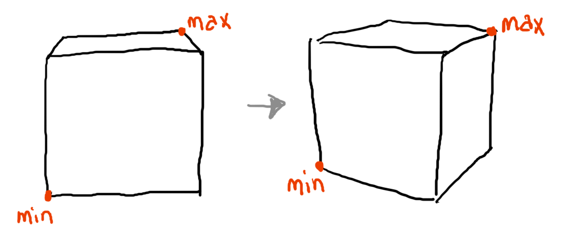
If you construct a new bounding box using only the transformed min and max points, check out what happens:
The behavior we expect is that the transformed box ought to be able to contain the volume of the rotated cube, but as you can see, that's not what happens here. It's gone all skinny, and definitely no longer contains all the volume of the original cube. This is because rotating an AABB means it is no longer axis-aligned! A new axis-aligned bounding box needs to be computed for that rotated box.
The right way to do this is to actually transform the points at all eight corners of the cube, and then find a new bounding box that contains all eight transformed points. In pseudocode, it might look something like this:
function transform(bbox, matrix)
  let p1 ← bbox.min
  let p2 ← point(bbox.min.x, bbox.min.y, bbox.max.z)
  let p3 ← point(bbox.min.x, bbox.max.y, bbox.min.z)
  let p4 ← point(bbox.min.x, bbox.max.y, bbox.max.z)
  let p5 ← point(bbox.max.x, bbox.min.y, bbox.min.z)
  let p6 ← point(bbox.max.x, bbox.min.y, bbox.max.z)
  let p7 ← point(bbox.max.x, bbox.max.y, bbox.min.z)
  let p8 ← bbox.max

  let new_bbox ← bounding_box(empty)

  for p in (p1, p2, p3, p4, p5, p6, p7, p8)
    add (matrix * p) to new_bbox
  end for

  return new_bbox
end function
Doing this ensures that the new bounding box is sufficiently large to hold the original cube after rotation.
Got that all passing? Awesome! You're finally ready to wrap some bounding boxes around aggregate shapes like groups and CSG objects. Read on!
Bounds for groups and CSG
So, now that you can transform a bounding box, you can implement a function for reporting a shape's bounds in the space of the shape's parent.
shapes.featureScenario: Querying a shape's bounding box in its parent's space
  Given shape ← sphere()
    And set_transform(shape, translation(1, -3, 5) * scaling(0.5, 2, 4))
  When box ← parent_space_bounds_of(shape)
  Then box.min = point(0.5, -5, 1)
    And box.max = point(1.5, -1, 9)
This is accomplished by transforming the shape's bounding box by the shape's transformation matrix.
function parent_space_bounds_of(shape)
  return transform(bounds_of(shape), shape.transform)
end function
With that function in hand, you're ready to find the bounds of a Group object. The following test sets up a group with a transformed sphere and cylinder, and shows that the bounds of the group are sufficient to include the child shapes.
groups.featureScenario: A group has a bounding box that contains its children
  Given s ← sphere()
    And set_transform(s, translation(2, 5, -3) * scaling(2, 2, 2))
    And c ← cylinder()
    And c.minimum ← -2
    And c.maximum ← 2
    And set_transform(c, translation(-4, -1, 4) * scaling(0.5, 1, 0.5))
    And shape ← group()
    And add_child(shape, s)
    And add_child(shape, c)
  When box ← bounds_of(shape)
  Then box.min = point(-4.5, -3, -5)
    And box.max = point(4, 7, 4.5)
CSG objects, being aggregate shapes like groups, should behave the same way, by reporting a bounding box sufficiently large to inculde their children.
csg.featureScenario: A CSG shape has a bounding box that contains its children
  Given left ← sphere()
    And right ← sphere() with:
      | transform | translation(2, 3, 4) |
    And shape ← csg("difference", left, right)
  When box ← bounds_of(shape)
  Then box.min = point(-1, -1, -1)
    And box.max = point(3, 4, 5)
Make these two tests pass by implementing the bounds_of(shape) function for each of Group and CSG. Both functions must find the parent-space bounds of each child object, and then merge them all together into a single bounding box. Here's the pseudocode for the Group version, to get you started:
function bounds_of(group)
  let box ← bounding_box(empty)

  for each child of group
    let cbox ← parent_space_bounds_of(child)
    add cbox to box
  end for

  return box
end function
Got that? Great! Next up, you'll do a handy bit of refactoring to be able to intersect rays with these bounding boxes.
Intersecting a bounding box
Having a bounding box for every shape in your ray tracer is great and all, but it won't do you any good unless you also teach your ray tracer how to see if a ray intersects those boxes. Fortunately, you've already implemented this feature!
Well, almost.
Back in chapter 12, "Cubes", of The Ray Tracer Challenge, you wrote some code that tests a ray against an axis-aligned bounding box (specifically, a cube) centered at the origin. For this section, you'll take that code and refactor it slightly so that it works with AABB's of any dimension and position.
Start with the following test, which tests the intersection between a ray and a cube-shaped AABB at the origin.
bounds.featureScenario Outline: Intersecting a ray with a bounding box at the origin
  Given box ← bounding_box(min=point(-1, -1, -1) max=point(1, 1, 1))
    And direction ← normalize(<direction>)
    And r ← ray(<origin>, direction)
  Then intersects(box, r) is <result>

  Examples:
    | origin            | direction        | result |
    | point(5, 0.5, 0)  | vector(-1, 0, 0) | true   |
    | point(-5, 0.5, 0) | vector(1, 0, 0)  | true   |
    | point(0.5, 5, 0)  | vector(0, -1, 0) | true   |
    | point(0.5, -5, 0) | vector(0, 1, 0)  | true   |
    | point(0.5, 0, 5)  | vector(0, 0, -1) | true   |
    | point(0.5, 0, -5) | vector(0, 0, 1)  | true   |
    | point(0, 0.5, 0)  | vector(0, 0, 1)  | true   |
    | point(-2, 0, 0)   | vector(2, 4, 6)  | false  |
    | point(0, -2, 0)   | vector(6, 2, 4)  | false  |
    | point(0, 0, -2)   | vector(4, 6, 2)  | false  |
    | point(2, 0, 2)    | vector(0, 0, -1) | false  |
    | point(0, 2, 2)    | vector(0, -1, 0) | false  |
    | point(2, 2, 0)    | vector(-1, 0, 0) | false  |
The intersects(box, ray) function returns a boolean value here. This is because (for the purposes of this feature) you don't need to know exactly where the bounding box is intersected, just whether or not it was. However, if you care about reusing code (and you should!), and you'd like your cube's local_intersect() function to be able to share this logic, you'll need to allow the function to report where the intersections occur. For this bonus chapter, though, the tests will only worry about true and false return values.
You can make that test pass by (re)using the logic from your cube's local_intersect() function. The next test, though, will require you to "massage" that code a bit, so that it can work with a bounding box that is not centered at the origin, and is not a perfect cube.
bounds.featureScenario Outline: Intersecting a ray with a non-cubic bounding box
  Given box ← bounding_box(min=point(5, -2, 0) max=point(11, 4, 7))
    And direction ← normalize(<direction>)
    And r ← ray(<origin>, direction)
  Then intersects(box, r) is <result>

  Examples:
    | origin           | direction        | result |
    | point(15, 1, 2)  | vector(-1, 0, 0) | true   |
    | point(-5, -1, 4) | vector(1, 0, 0)  | true   |
    | point(7, 6, 5)   | vector(0, -1, 0) | true   |
    | point(9, -5, 6)  | vector(0, 1, 0)  | true   |
    | point(8, 2, 12)  | vector(0, 0, -1) | true   |
    | point(6, 0, -5)  | vector(0, 0, 1)  | true   |
    | point(8, 1, 3.5) | vector(0, 0, 1)  | true   |
    | point(9, -1, -8) | vector(2, 4, 6)  | false  |
    | point(8, 3, -4)  | vector(6, 2, 4)  | false  |
    | point(9, -1, -2) | vector(4, 6, 2)  | false  |
    | point(4, 0, 9)   | vector(0, 0, -1) | false  |
    | point(8, 6, -1)  | vector(0, -1, 0) | false  |
    | point(12, 5, 4)  | vector(-1, 0, 0) | false  |
Your current check_axis() function (from the "Cubes" chapter), assumes that the cube extends from -1 to 1 along each axis, so it hard codes -1 and 1. To make it work for this more general algorithm, you'll need to pass the minimum and maximum extents of the bounding box for the axis in question. The following pseudocode adds the min and max parameters to the function. Careful, though: these are not the same as the min and max points of your bounding box. For this function, they are floating point values, just the x or y or z components from those points.
function check_axis(origin, direction, min, max)
  tmin_numerator = (min - origin)
  tmax_numerator = (max - origin)
...
The intersect function, then, sends the minimum and maximum values with each invocation of check_axis(), like this:
xtmin, xtmax ← check_axis(ray.origin.x, ray.direction.x, min.x, max.x)
# and so forth for y and z axes
With those changes, your tests should all be passing. You're ready now to plug this in and make it all work together.
Using the bounding box as an optimization
Once you can intersect a ray with a bounding box, you can put them to work. The main idea of this optimization is that when you need to see if a ray intersects a Group or CSG shape, you first check the ray against the bounding box of the Group or CSG. If (and only if) the ray intersects the bounding box, you then proceed to check the ray against the children of the Group or CSG.
These two tests demonstrate how it works with Group. They both use the test_shape() function you implemented in chapter 9, "Planes", and take advantage of the fact that the test shape will store a reference to the ray that it was intersected with. This way, if the saved ray is not set, then you know that no intersection was attempted against that shape.
groups.featureScenario: Intersecting ray+group doesn't test children if box is missed
  Given child ← test_shape()
    And shape ← group()
    And add_child(shape, child)
    And r ← ray(point(0, 0, -5), vector(0, 1, 0))
  When xs ← intersect(shape, r)
  Then child.saved_ray is unset

Scenario: Intersecting ray+group tests children if box is hit
  Given child ← test_shape()
    And shape ← group()
    And add_child(shape, child)
    And r ← ray(point(0, 0, -5), vector(0, 0, 1))
  When xs ← intersect(shape, r)
  Then child.saved_ray is set
The same is true when testing whether the CSG shape takes advantage of its bounding box, but this time both the left and right children are checked.
csg.featureScenario: Intersecting ray+csg doesn't test children if box is missed
  Given left ← test_shape()
    And right ← test_shape()
    And shape ← csg("difference", left, right)
    And r ← ray(point(0, 0, -5), vector(0, 1, 0))
  When xs ← intersect(shape, r)
  Then left.saved_ray is unset
    And right.saved_ray is unset

Scenario: Intersecting ray+csg tests children if box is hit
  Given left ← test_shape()
    And right ← test_shape()
    And shape ← csg("difference", left, right)
    And r ← ray(point(0, 0, -5), vector(0, 0, 1))
  When xs ← intersect(shape, r)
  Then left.saved_ray is set
    And right.saved_ray is set
In pseudocode, the local_intersect() function for both the Group and CSG shapes should be modified to look something like this:
function local_intersect(shape, ray)
  if intersects(bounds_of(shape), ray)
    # perform the usual intersection logic
    # ...
  else
    # nothing intersected
    return ()
  end if
end function
Awesome! With that in place, we can revisit that first illustration, with a thousand spheres arranged in a cube. Putting all thousand spheres into a single group will make it so that any ray that misses the group's bounding box will trivially miss all those spheres, too, and will give the scene a bit of a boost. You can do even better if you use eight groups (of 5x5x5 spheres each) instead of a single group.
Go ahead and try rendering something complex, like a model with a few thousand triangles in it, and see what kind of speed-up you get from this. Your renderer will still bog down when a ray intersects the model's bounding box, because it will need to test all those thousands of triangles, but it should still be significantly faster than without the bounding box.
It can, however, be better. Let's finish the bonus chapter off with a little chat about bounding volume hierarchies.
Bounding Volume Hierarchies (BVH)
So, you've got a group, and the group contains a few thousand shapes. Maybe they're triangles. I don't know. It doesn't really matter.
The bounding box around the group helps. It means that any ray that misses the bounding box won't have to be tested against any of those thousands of shapes. However, once the ray intersects the box, all bets are off.
So...what if you were to take all the children of that group, and divide them into two subgroups? Now, if the ray hits the outermost group, it will be tested against the group's two children—those two subgroups—each of which has its own bounding box.
Let's take it even further: what if you were to subdivide each of those subgroups in half again? In fact, just keep subdividing, chopping each group in half and partitioning the children based on which half they belong to. You wind up with a tree structure, groups containing groups, all the way down to the leaf nodes.
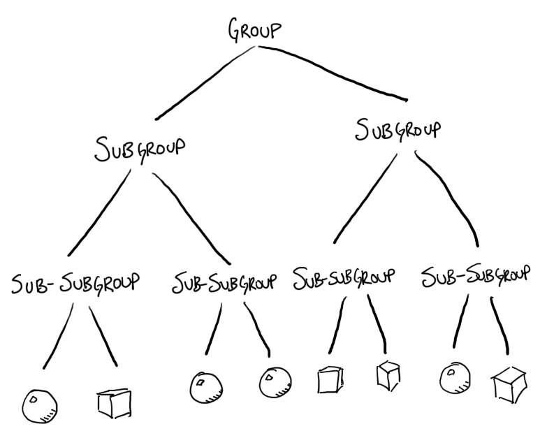
This is what is meant by a bounding volume hierarchy, or BVH. It's a hierarchy of these groups, each with a bounding box describing a smaller and smaller subset of the whole.
There are lots of ways to optimize large scenes. A BVH is only one of them. Other things you might read about are binary space partitioning (or BSP), quadtrees, octrees, and more. They all have different strengths and weaknesses. For this chapter, we're focusing solely on BVH's, but once you're done here, you should definitely go research some of the other techniques, too!
You're going to finish off this chapter by implementing a (relatively naive) BVH using groups and bounding boxes. It'll have plenty of room for improvement, but should still be enough to give your renders significantly more speed. The process will go like this:
- Split a bounding box into two equal halves.
- Partition the children of a group into appropriate subgroups.
- Recursively divide
GroupandCSGobjects.
Almost done. Here we go!
Splitting a bounding box
For this feature, you're going to implement splitting in the least-complicated way. You're not going to worry about how the objects are distributed within the bounding box, or anything like that—you'll just split the box geometrically in half, perpendicular to one of the three axes, x, y, or z.
The following tests introduce a new function, split_bounds(box), which returns two non-overlapping bounding boxes that cover the same volume as the original bounding box. Generally, you'll split whichever axis is longest. In the case of a perfect cube, though, let's just say you'll split it perpendicular to the x axis, as shown in this test with a 10x10x10 cube.
bounds.featureScenario: Splitting a perfect cube
  Given box ← bounding_box(min=point(-1, -4, -5) max=point(9, 6, 5))
  When (left, right) ← split_bounds(box)
  Then left.min = point(-1, -4, -5)
    And left.max = point(4, 6, 5)
    And right.min = point(4, -4, -5)
    And right.max = point(9, 6, 5)
When there is a longer axis, though, you'll spilt perpendicular to that one. The following three tests show how split_bounds() works when the bounding box is longest along any of the three axes.
bounds.featureScenario: Splitting an x-wide box
  Given box ← bounding_box(min=point(-1, -2, -3) max=point(9, 5.5, 3))
  When (left, right) ← split_bounds(box)
  Then left.min = point(-1, -2, -3)
    And left.max = point(4, 5.5, 3)
    And right.min = point(4, -2, -3)
    And right.max = point(9, 5.5, 3)

Scenario: Splitting a y-wide box
  Given box ← bounding_box(min=point(-1, -2, -3) max=point(5, 8, 3))
  When (left, right) ← split_bounds(box)
  Then left.min = point(-1, -2, -3)
    And left.max = point(5, 3, 3)
    And right.min = point(-1, 3, -3)
    And right.max = point(5, 8, 3)

Scenario: Splitting a z-wide box
  Given box ← bounding_box(min=point(-1, -2, -3) max=point(5, 3, 7))
  When (left, right) ← split_bounds(box)
  Then left.min = point(-1, -2, -3)
    And left.max = point(5, 3, 2)
    And right.min = point(-1, -2, 2)
    And right.max = point(5, 3, 7)
Here's one way to implement the split_bounds() function:
function split_bounds(box)
  # figure out the box's largest dimension
  dx ← size of box in x
  dy ← size of box in y
  dz ← size of box in z

  greatest ← maximum of dx, dy, dz

  # variables to help construct the points on
  # the dividing plane
  (x0, y0, z0) ← (x, y, z) from box.min
  (x1, y1, z1) ← (x, y, z) from box.max

  # adjust the points so that they lie on the
  # dividing plane
  if greatest = dx then
    x0 ← x1 ← x0 + dx / 2.0
  else if greatest = dy then
    y0 ← y1 ← y0 + dy / 2.0
  else
    z0 ← z1 ← z0 + dz / 2.0
  end if

  mid_min ← point(x0, y0, z0)
  mid_max ← point(x1, y1, z1)

  # construct and return the two halves of
  # the bounding box
  left ← bounding_box(min=box.min max=mid_max)
  right ← bounding_box(min=mid_min max=box.max)

  return (left, right)
end function
This works by figuring out which axis is the longest (by comparing greatest with the dx, dy, and dz variables) and then setting the minimum and maximum values for that axis to the midpoint between them. The mid_min and mid_max points represent opposite corners of the square on the dividing plane, which are then used to construct the new bounding boxes.
Once those tests are passing, you can move to the next part: partitioning the children of a group.
Partitioning children into subgroups
So, you've divided your bounding box in half. The thing you'll quickly discover is that there's a good chance that not all of the objects in the original group will fit in one or the other of the new bounding boxes. Consider the following illustration:

You could try and figure out how to tesselate that sphere in the middle into triangles, and then split the triangles that intersect the bounding box boundaries, and yeah, that would probably make a great science project and you'd learn a ton, but for this chapter...nah. Let's take a shortcut.
Instead of trying to force every object into one of the two bounding boxes, we'll let those that don't fit just be their best selves. We'll only partition those shapes that fit neatly into the two new bounding boxes.
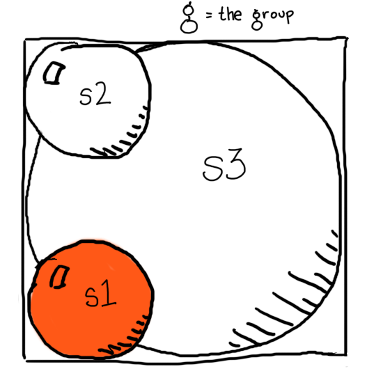
The following test illustrates this with a new function, partition_children(group). It returns two lists, or "buckets", containing the children that fit into the corresponding halves of the group's bounding box. The children that are placed into those buckets are removed from group, as well.
groups.featureScenario: Partitioning a group's children
  Given s1 ← sphere() with:
      | transform | translation(-2, 0, 0) |
    And s2 ← sphere() with:
      | transform | translation(2, 0, 0) |
    And s3 ← sphere()
    And g ← group() of [s1, s2, s3]
  When (left, right) ← partition_children(g)
  Then g is a group of [s3]
    And left = [s1]
    And right = [s2]
Here's what that test is doing. The first two spheres, s1 and s2, are translated so they fit into the left and right halves of the group's bounding box. The third, s3, sits in the middle, overlapping both halves. The resulting buckets contain s1 and s2, but not s3.
Once you have those two buckets, left and right, you can construct subgroups of them. The following test demonstrates this with a new function, make_subgroup(group, list).
groups.featureScenario: Creating a sub-group from a list of children
  Given s1 ← sphere()
    And s2 ← sphere()
    And g ← group()
  When make_subgroup(g, [s1, s2])
  Then g.count = 1
    And g[0] is a group of [s1, s2]
The make_subgroup() function creates a new subgroup and then adds each element of list to it. The subgroup is then added to group.
You're almost there. It's practically the home stretch!
Dividing groups into subgroups
Group subdivision works recursively, splitting a group and then splitting each of the children of the group, all the way down until there's nothing left to divide. To facilitate this, you'll first implement divide() on the leaf nodes—the primitive shapes—before implementing it on Group, and then on CSG.
The divide() function accepts two arguments: the shape to divide, and a threshold value. This threshold value only makes sense for groups, because it indicates the minimum number of children a group ought to have before it will be divided. A group with fewer children than the threshold will not be split (though it's children might be, if they themselves have more children than the threshold).
This means that for primitive shapes, the threshold value is effectively ignored. Further, since we've already decided that the primitive shapes in your ray tracer are not divisible, the divide() function will do nothing at all! Here's a test showing this, using a threshold of 1 to emphasize that even with the most eager of settings, the primitive shapes will not be modified.
shapes.featureScenario: Subdividing a primitive does nothing
  Given shape ← sphere()
  When divide(shape, 1)
  Then shape is a sphere
For a Group object, though, that threshold value plays a more important part. If the threshold is less than or equal to the number of children in the group, the children are partioned and corresponding subgroups formed and added to the group. Then, divide() is invoked on each of the group's children.
To illustrate this behavior, imagine a group containing three spheres, s1, s2, and s3.
The following test implements this configuration, and invokes the divide() function with a threshold of 1.
groups.featureScenario: Subdividing a group partitions its children
  Given s1 ← sphere() with:
      | transform | translation(-2, -2, 0) |
    And s2 ← sphere() with:
      | transform | translation(-2, 2, 0) |
    And s3 ← sphere() with:
      | transform | scaling(4, 4, 4) |
    And g ← group() of [s1, s2, s3]
  When divide(g, 1)
  Then g[0] = s3
    And subgroup ← g[1]
    And subgroup is a group
    And subgroup.count = 2
    And subgroup[0] is a group of [s1]
    And subgroup[1] is a group of [s2]
Because the threshold is less than (or equal to) the number of g's children, the children will be partitioned and sorted into subgroups when divide() is invoked. Then, divide() is invoked on each of the group's children.
In pseudocode, the divide() function looks something like this:
function divide(group, threshold)
  if threshold <= group.count then
    (left, right) ← partition_children(group)
    if left is not empty then make_subgroup(group, left)
    if right is not empty then make_subgroup(group, right)
  end if

  for each child in group
    divide(child, threshold)
  end for
end function
Note that even if the threshold is greater than the number of children in the group, and the group's immediate children are not partitioned, the divide() call is still propagated to the group's children.
The following test demonstrates this case by constructing a group g with two children, subgroup and s4. The subgroup child is a group with three children, s1, s2, and s3.
groups.featureScenario: Subdividing a group with too few children
  Given s1 ← sphere() with:
      | transform | translation(-2, 0, 0) |
    And s2 ← sphere() with:
      | transform | translation(2, 1, 0) |
    And s3 ← sphere() with:
      | transform | translation(2, -1, 0) |
    And subgroup ← group() of [s1, s2, s3]
    And s4 ← sphere()
    And g ← group() of [subgroup, s4]
  When divide(g, 3)
  Then g[0] = subgroup
    And g[1] = s4
    And subgroup.count = 2
    And subgroup[0] is a group of [s1]
    And subgroup[1] is a group of [s2, s3]
When the group is divided, a threshold of 3 is specified, but since g has fewer than 3 children, nothing happens to g itself. Regardless, though, the divide() call is propagated to g's children, and subgroup gets subdivided.
Dividing CSG shapes
There's just one more shape to which you need to add support for divide(): the CSG shape. In this case the divide() function does nothing to the shape itself, but, propagates the call to the shape's children.
The following test demonstrates this with a CSG shape consisting of two groups, each containing two spheres. After calling divide() on the CSG shape, the left and right children will have been split into two subgroups.
csg.featureScenario: Subdividing a CSG shape subdivides its children
  Given s1 ← sphere() with:
      | transform | translation(-1.5, 0, 0) |
    And s2 ← sphere() with:
      | transform | translation(1.5, 0, 0) |
    And left ← group() of [s1, s2]
    And s3 ← sphere() with:
      | transform | translation(0, 0, -1.5) |
    And s4 ← sphere() with:
      | transform | translation(0, 0, 1.5) |
    And right ← group() of [s3, s4]
    And shape ← csg("difference", left, right)
  When divide(shape, 1)
  Then left[0] is a group of [s1]
    And left[1] is a group of [s2]
    And right[0] is a group of [s3]
    And right[1] is a group of [s4]
And that's it! If all your tests are passing, you've just implemented a bounding volume hierarchy.
Wrapping it up
It's time to put your code to the test. Here are some ideas for you to try, to see how your renderer does now that you can build a BVH for complex scenes.
- Find an OBJ file online containing thousands of triangles, import it into your ray tracer, call
divide()on it, and render away. - Programmatically generate a 10x10x10 cube of spheres. Make it even bigger if you want! Put them all in a group, and
divide()the group. - Try a scene with multiple complex models in it. Design a table and put several teapots on it. How does it do?
The biggest win that BVH's (or any other similar optimization) give you, though, is the freedom to experiment. Lower render times mean less waiting, and more opportunities to try new features and scenes.
Good luck!
Did you like what you read here? The book follows the same format! With extensive tests and pseudocode, it will walk you through writing a ray tracer of your very own, from scratch. Grab your copy today!
If you've already purchased my book: thank you, thank you, thank you! I hope you find the same satisfaction I've found in writing your own 3D renderer.
Reviews really do drive sales, though, so it would mean a lot to me if you could leave a review of the book somewhere: Amazon.com, Goodreads.com, Twitter, Facebook, your own personal website, or any other place where folks might come across your review.
Thanks!
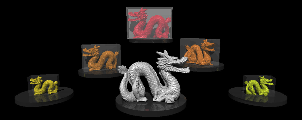
Each dragon in this scene consists of more than 24k triangles. Times six dragons, that comes out to more than 140k triangles in the scene. It really is not feasible to render without bounding boxes (or some similar optimization). Once you've implemented bounding boxes and BVH's, give the scene a try with your renderer!
You'll need the following dragon model, as well:
dragon.zip (607KB)
bounding-boxes.yml# ======================================================
# bounding-boxes.yml
#
# This file describes the banner image for the "Bounding
# boxes and hierarches" bonus chapter, at
#
# http://www.raytracerchallenge.com/bonus/bounding-boxes.html
#
# by Jamis Buck <jamis@jamisbuck.org>
# ======================================================

# ======================================================
# the camera
# ======================================================

- add: camera
  width: 500
  height: 200
  field-of-view: 1.2
  from: [0, 2.5, -10]
  to: [0, 1, 0]
  up: [0, 1, 0]

# ======================================================
# lights
# ======================================================

- add: light
  at: [-10, 100, -100]
  intensity: [1, 1, 1]

- add: light
  at: [0, 100, 0]
  intensity: [0.1, 0.1, 0.1]

- add: light
  at: [100, 10, -25]
  intensity: [0.2, 0.2, 0.2]

- add: light
  at: [-100, 10, -25]
  intensity: [0.2, 0.2, 0.2]

# ======================================================
# definitions
# ======================================================

- define: raw-bbox
  value:
    add: cube
    shadow: false
    transform:
      - [ translate, 1, 1, 1 ]
      - [ scale, 3.73335, 2.5845, 1.6283 ]
      - [ translate, -3.9863, -0.1217, -1.1820 ]

- define: dragon
  value:
    add: obj
    file: dragon.obj
    transform:
      - [ translate, 0, 0.1217, 0]
      - [ scale, 0.268, 0.268, 0.268 ]

- define: bbox
  value:
    add: raw-bbox
    transform:
      - [ translate, 0, 0.1217, 0]
      - [ scale, 0.268, 0.268, 0.268 ]

- define: pedestal
  value:
    add: cylinder
    min: -0.15
    max: 0
    closed: true
    material:
      color: [ 0.2, 0.2, 0.2 ]
      ambient: 0
      diffuse: 0.8
      specular: 0
      reflective: 0.2

# ======================================================
# scene
# ======================================================

- add: group
  transform:
    - [ translate, 0, 2, 0 ]
  children:
    - add: pedestal
    - add: group
      children:
        - add: dragon
          material:
            color: [ 1, 0, 0.1 ]
            ambient: 0.1
            diffuse: 0.6
            specular: 0.3
            shininess: 15
        - add: bbox
          material:
            ambient: 0
            diffuse: 0.4
            specular: 0
            transparency: 0.6
            refractive-index: 1

- add: group
  transform:
    - [ translate, 2, 1, -1 ]
  children:
    - add: pedestal
    - add: group
      transform:
        - [ rotate-y, 4 ]
        - [ scale, 0.75, 0.75, 0.75 ]
      children:
        - add: dragon
          material:
            color: [ 1, 0.5, 0.1 ]
            ambient: 0.1
            diffuse: 0.6
            specular: 0.3
            shininess: 15
        - add: bbox
          material:
            ambient: 0
            diffuse: 0.2
            specular: 0
            transparency: 0.8
            refractive-index: 1

- add: group
  transform:
    - [ translate, -2, .75, -1 ]
  children:
    - add: pedestal
    - add: group
      transform:
        - [ rotate-y, -0.4 ]
        - [ scale, 0.75, 0.75, 0.75 ]
      children:
        - add: dragon
          material:
            color: [ 0.9, 0.5, 0.1 ]
            ambient: 0.1
            diffuse: 0.6
            specular: 0.3
            shininess: 15
        - add: bbox
          material:
            ambient: 0
            diffuse: 0.2
            specular: 0
            transparency: 0.8
            refractive-index: 1

- add: group
  transform:
    - [ translate, -4, 0, -2 ]
  children:
    - add: pedestal
    - add: group
      transform:
        - [ rotate-y, -0.2 ]
        - [ scale, 0.5, 0.5, 0.5 ]
      children:
        - add: dragon
          material:
            color: [ 1, 0.9, 0.1 ]
            ambient: 0.1
            diffuse: 0.6
            specular: 0.3
            shininess: 15
        - add: bbox
          material:
            ambient: 0
            diffuse: 0.1
            specular: 0
            transparency: 0.9
            refractive-index: 1

- add: group
  transform:
    - [ translate, 4, 0, -2 ]
  children:
    - add: pedestal
    - add: group
      transform:
        - [ rotate-y, 3.3 ]
        - [ scale, 0.5, 0.5, 0.5 ]
      children:
        - add: dragon
          material:
            color: [ 0.9, 1, 0.1 ]
            ambient: 0.1
            diffuse: 0.6
            specular: 0.3
            shininess: 15
        - add: bbox
          material:
            ambient: 0
            diffuse: 0.1
            specular: 0
            transparency: 0.9
            refractive-index: 1

- add: group
  transform:
    - [ translate, 0, 0.5, -4 ]
  children:
    - add: pedestal
    - add: dragon
      material:
        color: [ 1, 1, 1 ]
        ambient: 0.1
        diffuse: 0.6
        specular: 0.3
        shininess: 15
      transform:
        - [ rotate-y, 3.1415 ]